Colors of analog camera

While writing the last post Analog Diary III, I realized that I did not like photos order that was only dictated by the photo number from the scanner. The image presentation was not smooth enough, and I was looking for a way to sort images based on their luminosity and dominant color so the gallery would have more visual flow.

To do it, I wrote a short Python script that would help me with that task. First, the imports:

import glob
import os
import shutil

import imageio as io
import matplotlib.pyplot as plt
import numpy as np

from sklearnex import patch_sklearn
patch_sklearn()

from sklearn.cluster import KMeans
from skimage.transform import rescale

I used some general Python libraries for file discovery (glob) and system tools (os and shutil). Other libraries are more sophisticated: imageio for image reading and writing, matplotlib for plotting, NumPy for general array operations, and sklearn to perform k-means clustering. In addition, I use the Intel accelerated sklearn library to make the k-means calculations ~10x faster. The last import is the sklearn-image library which allows per-image calculations. Next, let’s define some helper variables and functions:

img_paths = glob.glob('/home/dzyla-photo/content/blog/post36/images/*.*')
n_clusters = 10
dominant_color = []
colormap = np.zeros((20, 200, 3))

img_paths will store all the paths of the images, n_clusters is a number of dominant colors to find in the picture, dominant_color is the list that will keep those colors, and colormap will be used to visualize the dominant colors. Let’s do some per image calculations:

for file in img_paths:
  img = io.imread(file)

  img = rescale(img, (0.3, 0.3, 1))
  initial_shape = img.shape

  img = img.reshape(-1, 3)
  print(initial_shape)

  y_labels = KMeans(n_clusters=n_clusters, random_state=0).fit_predict(img)

This code uses imageio to open the image file from the path, followed by the skimage library that rescales the image to 30% of the original size but keeps the RGB channel dimension unchanged. We keep the initial image dimension as a variable and reshape the image to get the array of all pixels in one dimension. Next, using the k-means clustering, all pixels are grouped into 10 classes. Each pixel will belong to one of 10 classes (from 0 to 9). The next task is a little bit more complicated. All pixels belong to one of 10 classes, but because many pixels in one class will have different values, we need to calculate the average color per class:

color_list = []
clustered_img = np.zeros(img.shape)

for cluster in range(0, n_clusters):
  color = np.mean(img[y_labels == cluster], axis=0)
  color_list.append(color)
  clustered_img[y_labels == cluster] = color

Here, for each class, we calculate the average pixel value. We define an empty list that will hold calculated average colors and clustered_image, which will be an image with classified pixels substituted with calculated class colors. To do so, we select pixels that belong to the same class and average them. The result we add to the color_list. To calculate the clustered_img, the pixels corresponding to the given class are set to the average class color. Next, we will sort the obtained averaged colors per count:

color_label, color_frequency = np.unique(y_labels, return_counts=True)
sorting_order = np.argsort(color_frequency)

color_frequency = color_frequency[sorting_order]
color_list = np.array(color_list)[sorting_order]

From the y_labels class membership list, we calculate the unique values (that will be the class number from 0 to 9) together with the class count. This list will be ordered based on the values in the color_label array (0 -> 9). Thus, we need to sort the color_frequency array. np.argsort returns the array of indexes that will sort the original array, which is very useful in that case. We apply the sorting order to color_frequency and color_list arrays, resulting in two arrays ordered by the increasing population of the color in the picture. Now we have all elements ready to plot the colors according to their frequencies:

index = 0
color_map = np.zeros((20, initial_shape[1],3))

for n, color in enumerate(color_list):
    fraction = int(initial_shape[1] * (color_frequency[n] / img.shape[0]))
    if n < len(color_frequency) - 1:
        color_map[:, index:index + fraction] = color
    else:
        color_map[:, index:] = color
        dominant_color.append(color)
    index = index + fraction

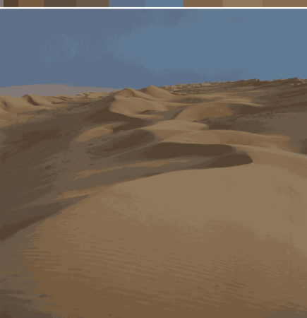
We define two new variables, the index will allow us to keep track of the array to plot colors, and color_map will be a bar plot of dominant colors in the picture. We iterate by sorting color_list, calculate the fraction of the image that belongs to the current class, and adjust it to the size of the source image. Due to the rounding error of each fraction, there will be some pixels that won’t be assigned to color; thus, we will use the most frequent color to fill missing pixels. For further calculations, we also keep the last color (the most frequent) in the dominant_color list. Finally, we move the index used to define the borders between colors. The above code will produce an image like this:

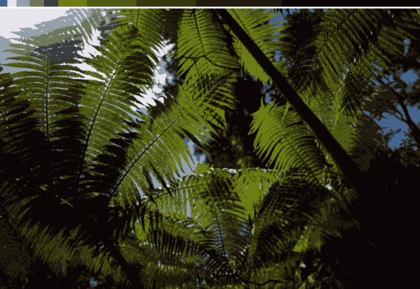
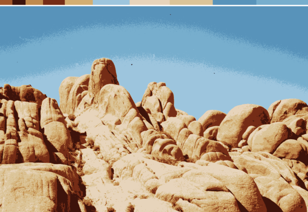
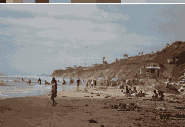
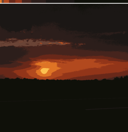
Let’s add the color distribution to the image that is reduced to 10 colors and plot it:

white_spacer = np.ones((5, initial_shape[1], 3))
final_img = np.concatenate((color_map, white_spacer, clustered_img.reshape(initial_shape)), axis=0)

plt.imshow(final_img)
plt.axis('off')
plt.tight_layout()
plt.savefig(os.path.basename(file).replace('.jpg', '_clustered.png').replace('JPG', '_clustered.png'),
            bbox_inches='tight', pad_inches=0)
plt.clf()

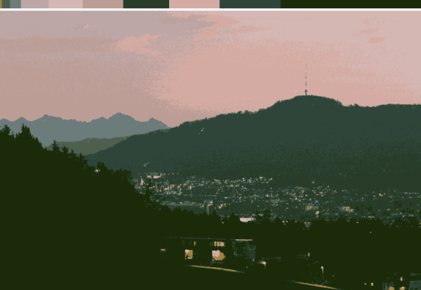
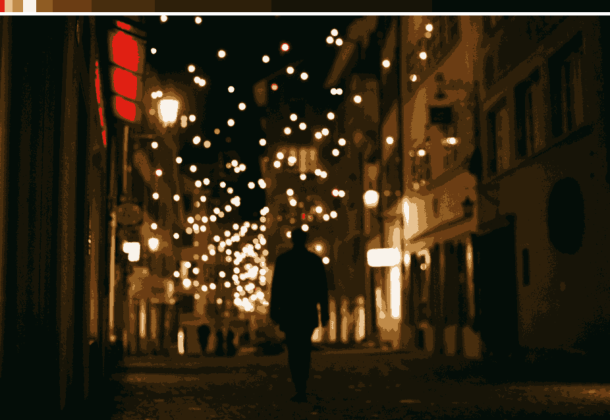
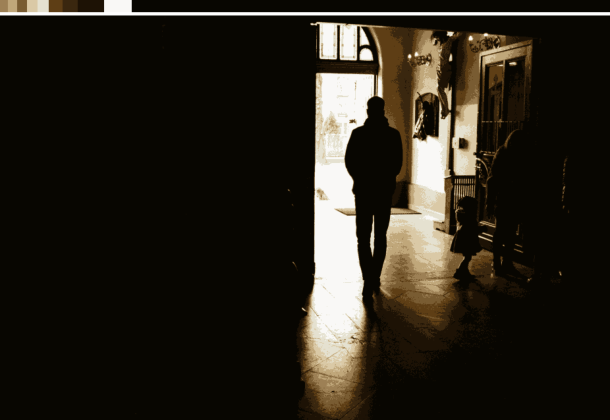
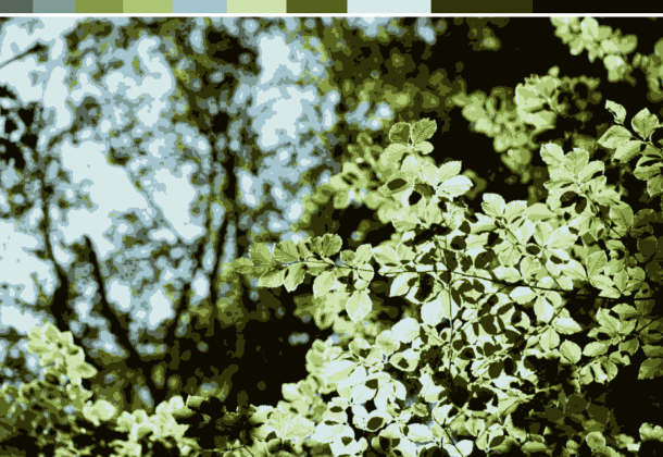
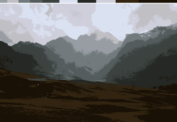
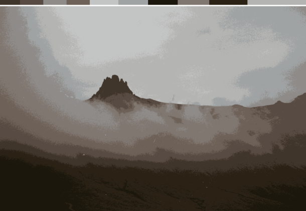
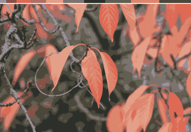
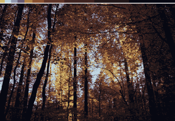
To separate the image from the color bar, we use a white spacer that is 5px high and image wide. Let’s combine all parts to get the final image by concatenating color_map, spacer, and image on the height axis. To generate two-dimensional images from a one-dimensional pixel array, we reshape this array back to its original shape. Plotting of the results is done in Matplotlib with disabled axes and a tight layout and, finally, save the image without white padding. The result for an example photo:

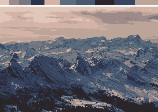
This ends the for loop and generates color-clustered images for all files in the folder. Using the information from the color distribution per image from the dominant_color list, it is possible to sort images based on their dominant color luminosity (from the great color tutorial from Alan Zucconi):

adjusted_sorted_colors = []
for color in dominant_color:
    adjusted_sorted_colors.append(np.sqrt(.241 * color[0] + .691 * color[1] + .068 * color[2]))

color_map = colormap
idx = np.linspace(0, color_map.shape[1], len(dominant_color) + 1, dtype=int)

img_order = np.argsort(adjusted_sorted_colors)

for n, color in enumerate(np.array(dominant_color)[img_order]):
    color_map[:, idx[n]:idx[n + 1]] = color

Let’s create an empty list again to store the color luminosity calculated according to the equation. Let’s copy the color_map empty array and define equal spacing on the long dimension. Then we sort the adjusted_sorted_colors based on their luminosity value and assign this color to fractions of the color_map. This will generate the final sorted color array (top unsorted, bottom sorted):

The final step is to change the names of the photos according to the sorted dominant color luminosity:

os.makedirs('sorted_imgs', exist_ok=True)
for n, file in enumerate(img_paths):
    shutil.copy2(file, './{}/{}_{}'.format('sorted_imgs', img_order[n], os.path.basename(file)))

Let’s create a folder called sorted_imgs and iterate through the image paths and, using shutil, copy the file to the sorted_imgs folder, changing the name by putting the consecutive number in from the file name. And that’s it! The result of this sorting is shown in the previous post Analog Diary III. The final and updated script can be found here:

Ok, so we have a way to sort images based on their dominant color luminosity. While going through the analog photos, I noticed that different films give different vibes and colors. The idea was born: let’s generate film-specific dominant color lists and see if there is something cool there!

During the past few years, I developed almost 40 films, including Kodak Portra, Kodak Gold, Kodak Ultramax, Ilford HP5, Agfa, Fujicolor, and Ektar. Of course, colors will depend on the subject, exposure, and many other factors but let’s check some most dominant color pallets per film. I will use part of the above script, but instead of calculating the dominant colors per image, I will load all images in the developed film folder and change them to a one-dimensional array of pixels. This massive array will be classified with K-means. Color maps from different films are presented below:

Kodak Portra 400 (Yashica Mat 124G, ~140 photos):

Ektar 100 (~80 photos):

Fujicolor Xtra 400 (~80 photos):

Kodak Ultramax 400 (~120 photos):

Ilford HP5 plus 400 (~115 photos):

Agfa 400 (~37 photos):

Fujifilm Superia 400 (~39 photos):

Fujicolor C200 (~80 photos):

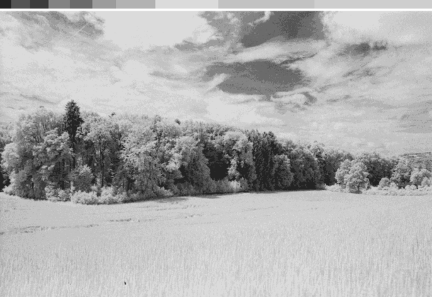
Rollei Infrared 400 (~30 photos):

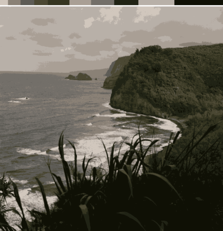
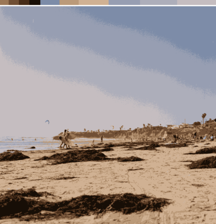
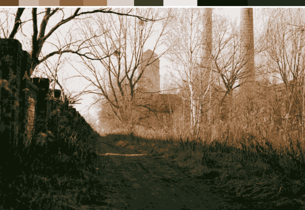
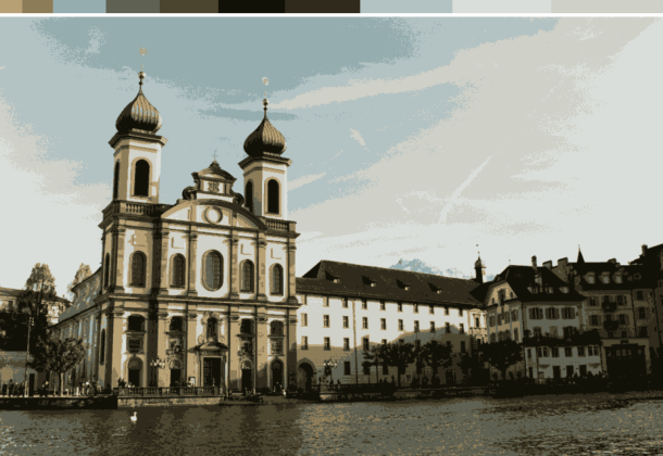
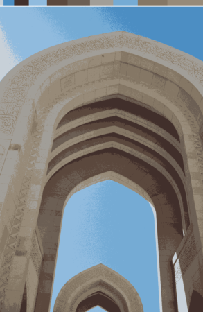
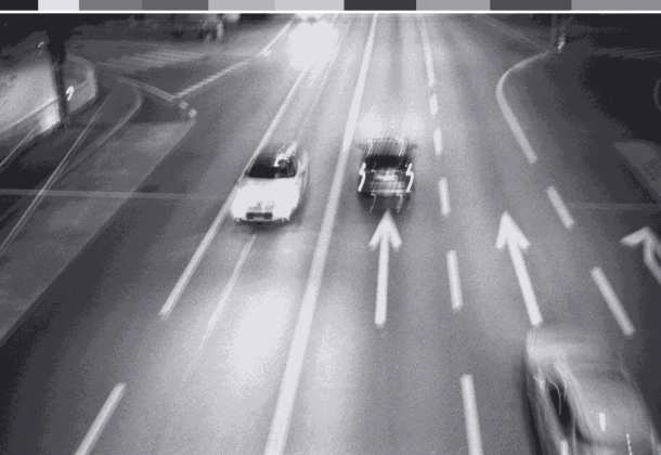
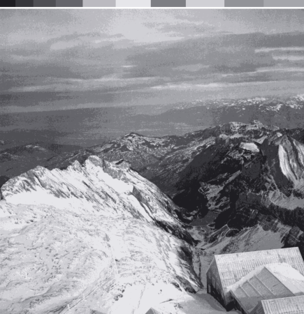
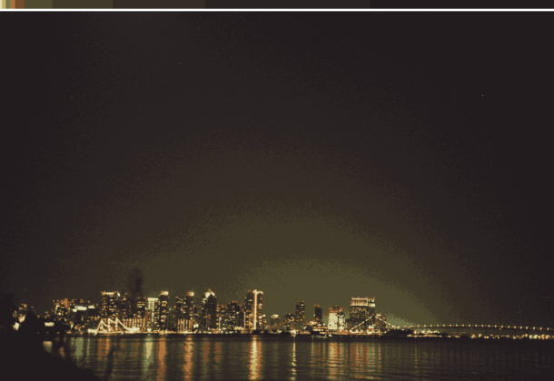
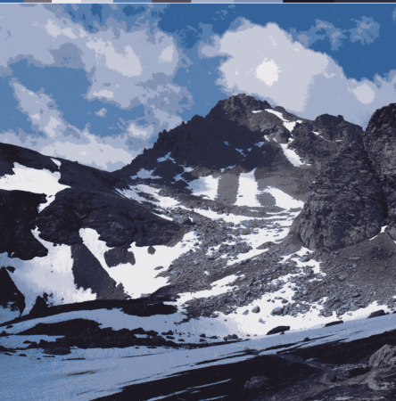
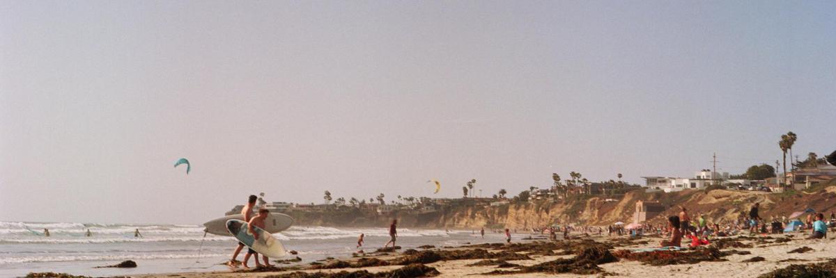
I must admit I like the colors obtained by clustering different films but can’t tell whether there is any color dependence on the film. Most likely, a considerably more sophisticated analysis would be required to fully see the palette difference between various films. Nevertheless, it was a fun project to do! More photos with their most dominant colors are below: