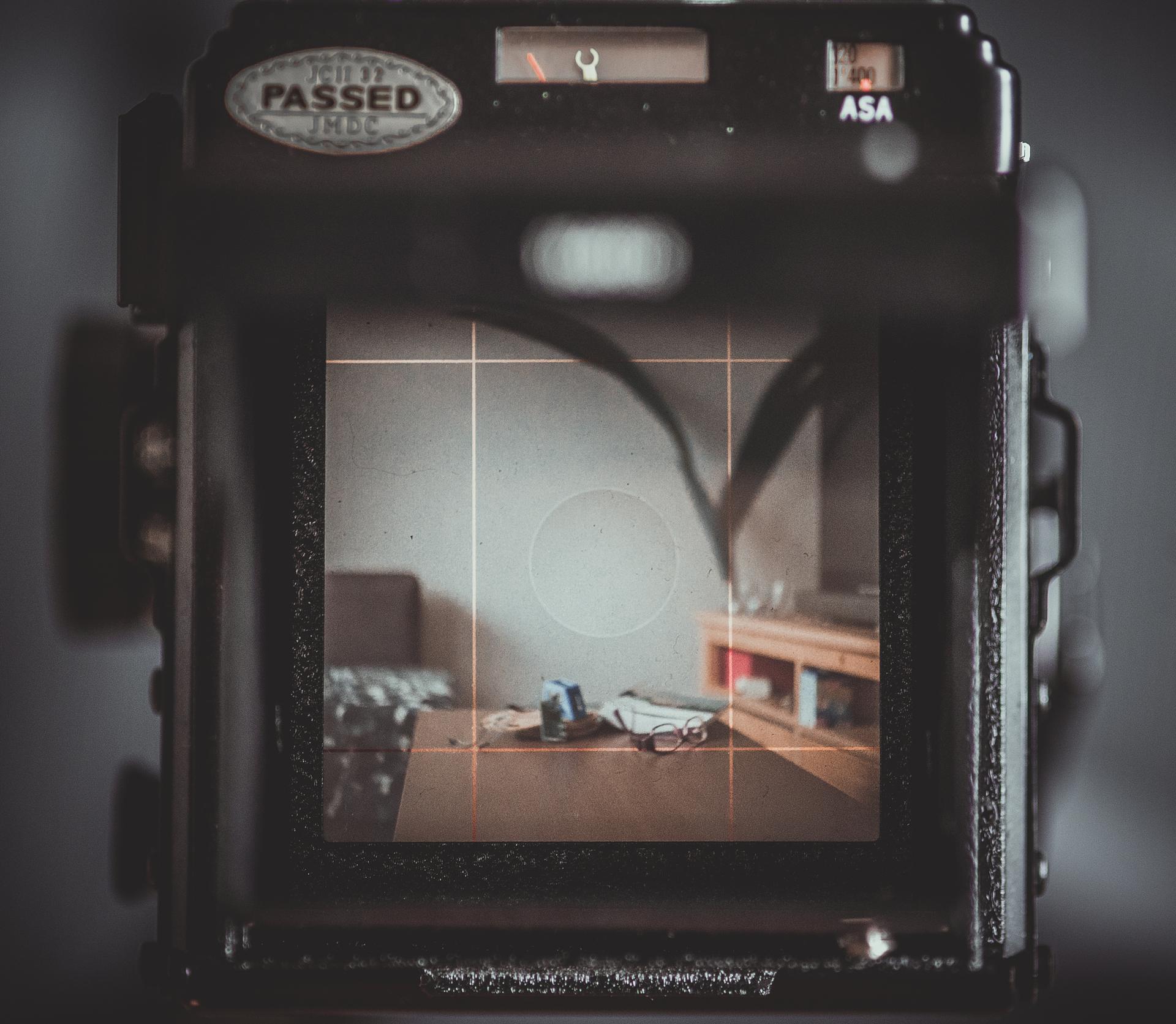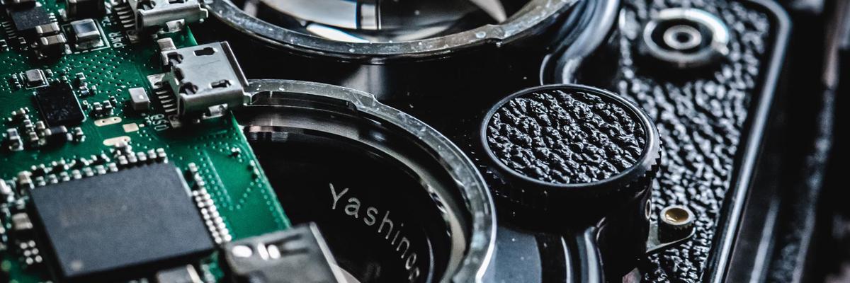
As soon as I bought my first medium format camera, Yashica MAT 124G I realized that there will have a problem with exposure meter. First of all, camera was released in 1970, so the light meter is not very accurate. Secondly, it uses mercury 1.35V batteries which are no longer available and only expensive and fast running out zinc-air batteries can be purchased. The last but not least, light meter is not backlit, thus it is almost impossible to guess the proper time and exposure settings in the dark environment. All this reasons convinced me to purchase an alternative light meter which would also calculate the exposure time and aperture number. However, besides commercially available light meters, which are rather expensive (>200$) there was nothing what would fill in the gap.
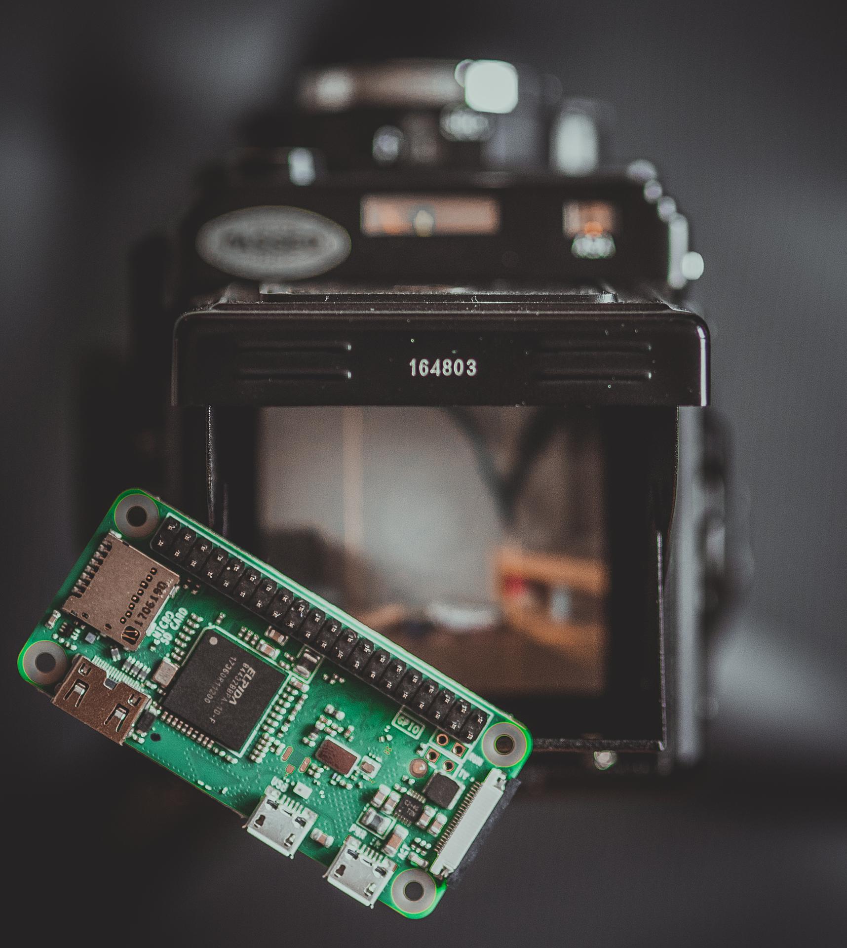
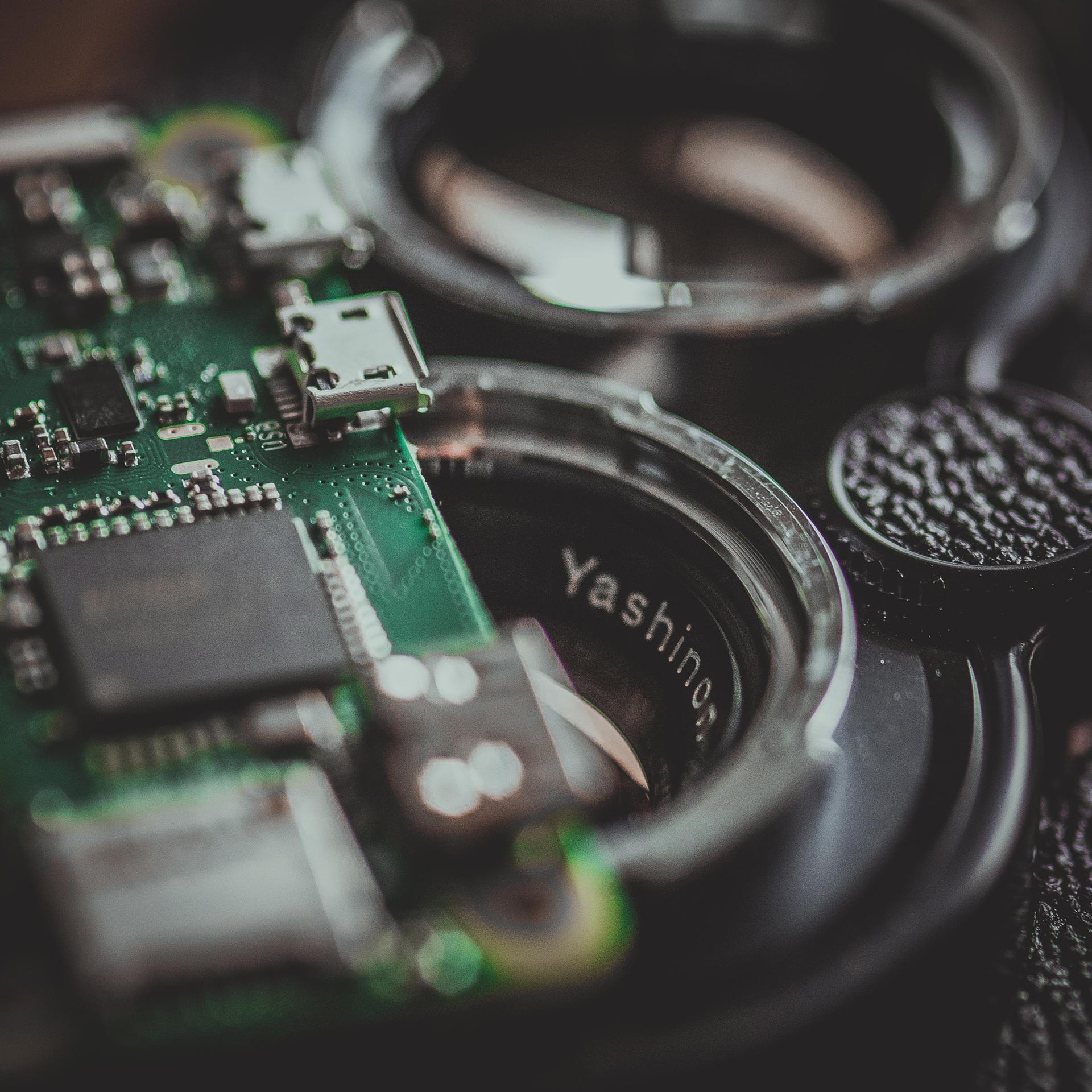
Short research on popular shopping websites gave me an alternative solution – why not to use Raspberry with light intensity sensor, couple this with a display and wire it up. The problem was, that my programming skills are rather basic and I also had no idea about photometry. But what is life without trying 😉 The Internet is the biggest invention indeed, and everything can be found there. After short research (this time the proper one) I have learned some things which I will try to explain here.
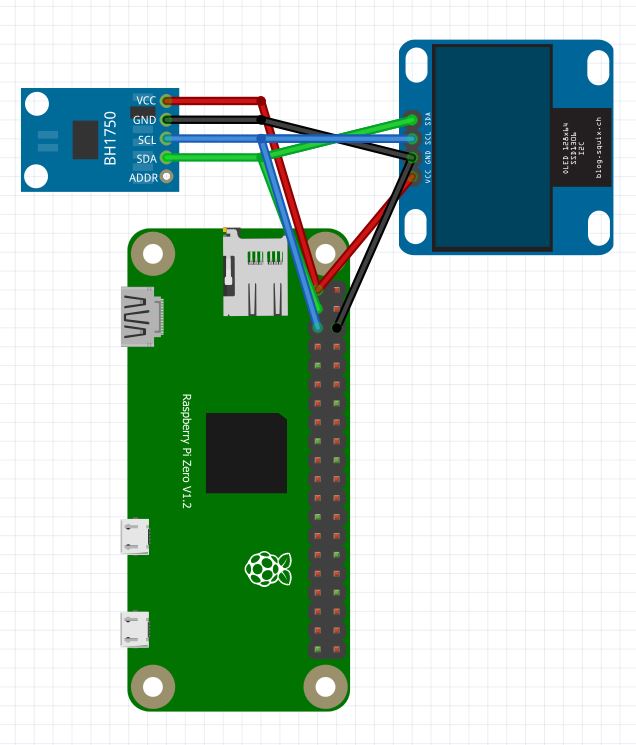
Sensor which I bought was GY-30 light intensity sensor for ~3$. It is connected through I2C bus to controller, which in this case is Raspberry Pi Zero W. There is publicly available python script which enables to measure the light intensity in lux. According to Wikipedia lux is an SI derived unit of illuminance and luminous emittance, measuring luminous flux per unit area, which means that it is amount of light per area. If the area is a camera sensor and we would sum the light over time (exposure time) we will get a picture. However, lux itself is not telling anything about the exposure (EV) which is required to calculate the ratio of exposure time and aperture. The dependency of lux and exposure (EV) is described with following equation:
$$ (eq. 1) \ \ lux=2^{EV}\cdot2.5 $$
This tell us that exposure is in the exponent – which basically means that every double intensity of the light would change the exposure only by 1. Plotting this dependency we would get:
import numpy as np
import matplotlib.pyplot as plt

x = np.arange(0.01,10000,1)

ev = np.log2(x/2.5)
print(np.log2(20/2.5))
plt.figure(figsize=(12,8))
plt.plot(x,ev)
plt.xlabel('Light intensity, lux', fontsize = 16)
plt.ylabel('Exposure (EV)', fontsize = 16)
plt.title('Dependence of Exposure on light intensity', fontsize = 16)

plt.annotate('0.1 lux - full moon in the night', xy=(0.1, -4.64), xytext=(600, -6),
            arrowprops=dict(arrowstyle="->",facecolor='black'))
plt.annotate('3 lux - twilight', xy=(3, 0.263), xytext=(1200, -3),
            arrowprops=dict(arrowstyle="->",facecolor='black'))
plt.annotate('30 lux - Dark urban surroundings', xy=(3.5849, 3.58), xytext=(1800, 0),
            arrowprops=dict(arrowstyle="->",facecolor='black'))
plt.annotate('100 lux - Very dark overcast day', xy=(100, 5.32), xytext=(2400, 3),
            arrowprops=dict(arrowstyle="->",facecolor='black'))
plt.annotate('500 lux - Very dark overcast day', xy=(500, 7.64), xytext=(3000, 6),
            arrowprops=dict(arrowstyle="->",facecolor='black'))
plt.annotate('1000 lux - Overcast day', xy=(1000, 8.64), xytext=(3600, 8),
            arrowprops=dict(arrowstyle="->",facecolor='black'))
plt.annotate('10000  lux < - Sunny day', xy=(9950, 11.96), xytext=(4200, 9.5),
            arrowprops=dict(arrowstyle="->",facecolor='black'))
plt.show()
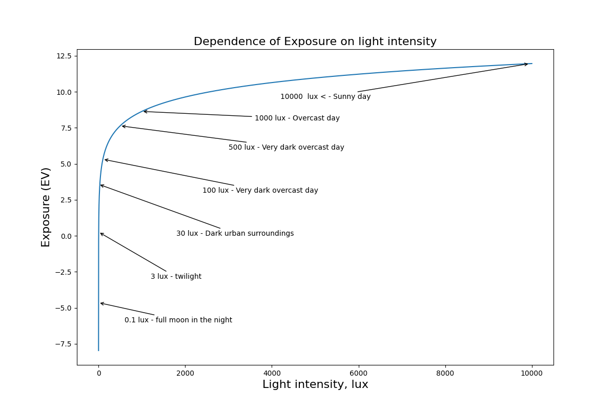
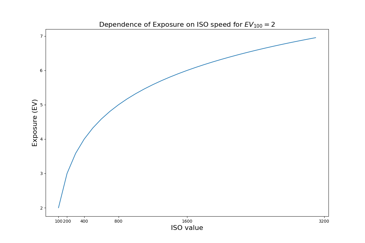
This plot also shows nicely that change of light intensity in lux is drastic (over 10k!), when exposure changes only slightly (from ~ -8 to 12). Obtained exposure can be already used for time and aperture calculations. There is only one variable missing: ISO – the sensitivity of the photosensitive element (film, CCD or CMOS matrix). EV is usually calculated for the default ISO value of 100. Exposure at various ISO can be calculated from the following equation:
$$ (eq. 2) \ \ EV_{ISO} = EV_{100} + log2 \left(\frac{ISO}{100}\right) $$
This means, that change of the ISO by one stop (from 100 to 200 for example) would increase the exposure measured at ISO 100 by 1 EV, for the visualization check the plot below.
import numpy as np
import matplotlib.pyplot as plt

ISO = np.arange(100,3200,100)
ev1 = 2
ev = ev1 + np.log2(ISO/100)
plt.figure(figsize=(12,8))

plt.plot(ISO,ev)
plt.xticks([100,200,400,800,1600,3200])

plt.xlabel('ISO value', fontsize = 16)
plt.ylabel('Exposure (EV)', fontsize = 16)
plt.title(r'Dependence of Exposure on ISO speed for $EV_{100} = 2$', fontsize = 16)

plt.show()
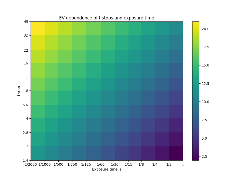
Now, having the connection between the signal from sensor and exposure, as well as exposure dependence on ISO we can go further. It is not so obvious that for single EV we can describe multiple camera settings. This is because the dependence of N (aperture number) and t (exposure time) is given as follows:
$$ (eq. 3) \ \ EV = log2 \left(\frac{N^{2}}{t}\right) $$ $$ (eq. 4) \ \ \frac{N^{2}}{t} = 2^{EV} $$
This means that as long as ratio
\(\frac{N^{2}}{t}\)
is constant, the exposure will stay the same. This dependency can be very nicely shown for most common apertures numbers and times as a 2D matrix:
import matplotlib.pyplot as plt
import numpy as np
from fractions import Fraction

# initialize list to keep values
times_frac = []

# Get the exposures
times = ['1','1/2','1/4','1/8','1/15','1/30' , '1/60','1/125', '1/250', '1/500', '1/1000', '1/2000']

# Convert exposures to floats
times_float = np.array([float(Fraction(x)) for x in times])

# Get the F-stops
f_stops= [1.4, 2, 2.8 , 4, 5.6, 8, 11, 16, 22, 32, 45]

def plot_matrix(iso):

    # set figure
    fig = plt.figure()
    ax = plt.subplot()

    # create a gridmesh with X -> times and Y f-stops
    X, Y = np.meshgrid(times_float, f_stops)

    # Create a value for each data point that equals the N^2/t
    R = Y**2 / X

    # iterate through all data points and calculate the exposure
    for idx_x, row in enumerate(R):
        for idx_y, element in enumerate(row):
            R[idx_x][idx_y] = (np.log2(element)+iso/100-1)

    # Setup plot
    ax.set_title('EV dependence of f stops and exposure time')
    ax.set_ylabel('f stop')
    ax.set_xlabel('Exposure time, s')
    ax.set_xscale('log')
    ax.set_xticks(times_float)
    ax.set_xticklabels(times)

    ax.set_yscale('log')
    ax.set_yticks(f_stops)
    ax.set_yticklabels(f_stops)

    graph = ax.pcolormesh(X, Y, R)
    fig.colorbar(graph, ax=ax)
    plt.show()

plot_matrix(200)
When all equations are already here, we can relate sensor readout in lux with
\(\frac{N^{2}}{t}\)
ratio. To do so, we couple equation 1, 2 and 4:
$$ (eq. 5) \ \ lux = 2^{EV} \cdot 2^{log2(\frac{ISO}{100})} \cdot 2.5 \leftrightarrow lux = 2^{EV} \cdot \frac{ISO}{100} \cdot 2.5 $$
$$ (eq. 6) \ \ lux = 2^{log2(\frac{N^{2}}{t})} \cdot \frac{ISO}{100} \cdot 2.5 \leftrightarrow lux = \frac{N^{2}}{t}\cdot \frac{ISO}{100} \cdot 2.5 $$ $$ (eq. 7) \frac{N^{2}}{t} = \frac{lux }{\frac{ISO}{100} \cdot 2.5} $$
to calculate aperture with given time:
$$ (eq. 8) \ \ t = \frac{N^{2} \cdot \frac{ISO}{100}}{lux} \cdot 2.5 $$
to calculate time with given aperture:
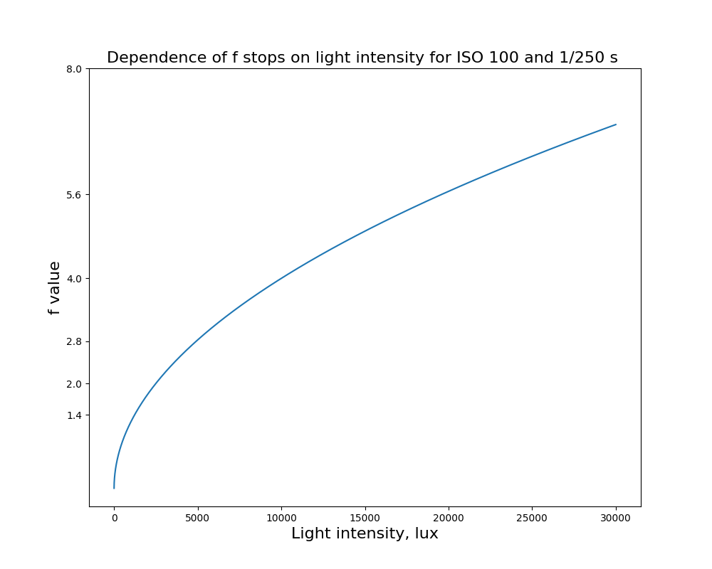
$$ (eq. 9) \ \ N = \sqrt{\frac{t \cdot lux}{\frac{ISO}{100} \cdot 2.5}} $$
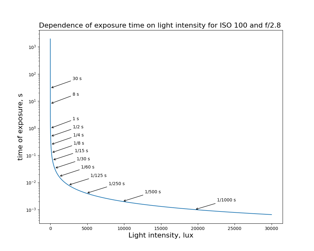
Because old cameras usually have fixed available exposure times and f stops, calculations are much easier. For my light meter I have chosen to calculate exposure time for fixed f stops: 1.4, 2, 2.8 , 4, 5.6, 8, 11, 16. The dependence of time and f stops can be checked at the graphs below.
import numpy as np
import matplotlib.pyplot as plt

lux = np.arange(0.01,30000,1)

iso=100
t = 1/250

n = np.sqrt((t*lux)/(iso/100*2.5))
print(n)

plt.figure(figsize=(10,8))
plt.plot(lux,n)
plt.yticks([1.4, 2, 2.8 , 4, 5.6, 8,])
plt.xlabel('Light intensity, lux', fontsize = 16)
plt.ylabel('f value', fontsize = 16)
plt.title(r'Dependence of f stops on light intensity for ISO 100 and 1/250 s ', fontsize = 16)
plt.show()
import numpy as np
import matplotlib.pyplot as plt

lux = np.arange(0.01,30000,1)

iso=100
n = 2.8

t = (n**2*(iso/100)*2.5)/lux

plt.figure(figsize=(10,8))
plt.plot(lux,t)
places = [30,8,1,1/2,1/4,1/8,1/15,1/30 , 1/60,1/125, 1/250, 1/500, 1/1000, 1/2000,1/4000]

times = ['30','8','1','1/2','1/4','1/8','1/15','1/30' , '1/60','1/125', '1/250', '1/500', '1/1000', '1/2000', '1/4000']
plt.yscale('log',basey=10)
plt.xlabel('Light intensity, lux', fontsize = 16)
plt.ylabel('time of exposure, s', fontsize = 16)
plt.title(r'Dependence of exposure time on light intensity for ISO 100 and f/2.8 ', fontsize = 16)

y = 1000

for w,i in enumerate(times):
    x = n**2/places[w]*2.5
    plt.annotate(str(times[w])+' s', xy=(x, places[w]), xytext=(x+3000, places[w]*2),
                 arrowprops=dict(arrowstyle="->", facecolor='black'))
    y+=1500

plt.show()
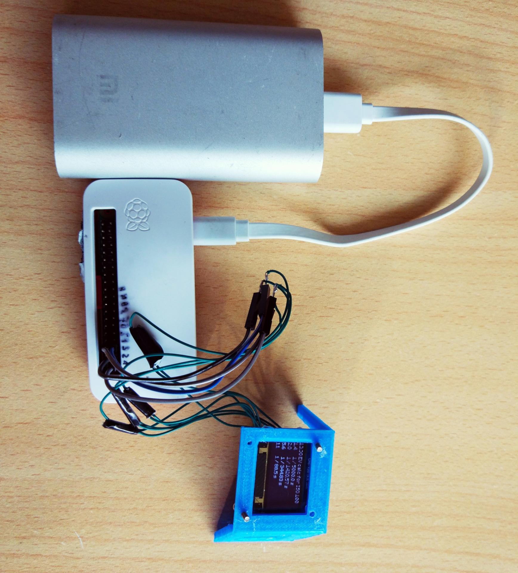
Having formula linking readout from Raspberry sensor and EV, I could put it all together. I used GY-30 light sensor python script and modified it to show exposure times for given f stops. Original script can be downloaded from here: www.raspberrypi-spy.co.uk/.
#!/usr/bin/python
import math
from time import sleep

import smbus

# Define some constants from the datasheet
DEVICE = 0x23  # Default device I2C address

POWER_DOWN = 0x00  # No active state
POWER_ON = 0x01  # Power on
RESET = 0x07  # Reset data register value

# Start measurement at 4lx resolution. Time typically 16ms.
CONTINUOUS_LOW_RES_MODE = 0x13
# Start measurement at 1lx resolution. Time typically 120ms
CONTINUOUS_HIGH_RES_MODE_1 = 0x10
# Start measurement at 0.5lx resolution. Time typically 120ms
CONTINUOUS_HIGH_RES_MODE_2 = 0x11
# Start measurement at 1lx resolution. Time typically 120ms
# Device is automatically set to Power Down after measurement.
ONE_TIME_HIGH_RES_MODE_1 = 0x20
# Start measurement at 0.5lx resolution. Time typically 120ms
# Device is automatically set to Power Down after measurement.
ONE_TIME_HIGH_RES_MODE_2 = 0x21
# Start measurement at 1lx resolution. Time typically 120ms
# Device is automatically set to Power Down after measurement.
ONE_TIME_LOW_RES_MODE = 0x23

bus = smbus.SMBus(1)  # Rev 2 Pi uses 1

def convertToNumber(data):
    # Simple function to convert 2 bytes of data
    # into a decimal number
    return ((data[1] + (256 * data[0])) / 1.2)

def readLight(addr=DEVICE):
    data = bus.read_i2c_block_data(addr, ONE_TIME_HIGH_RES_MODE_1)
    return convertToNumber(data)

def write_to_file(string):  # optional for export of the data
    import csv
    with open('light.csv', 'a') as fh:
        writer = csv.writer(fh)
        writer.writerow(string)

def iso_calc(iso):
    return 2 ** (math.log2(iso / 100))

def measure(iso):
    f_stops = [1.4, 2, 2.8, 4, 5.6, 8, 11, 16, 22, 32, 45]
    t_calc = []

    while True:  # continues measurement
        light = round(readLight(), 2)  # get the light value from sensor
        if light > 0:  #Only when light detected on the sensor
            for fstop in f_stops:  # calculate the time of exposure for all f/stops
                t_calc.append(round(2.5 * fstop ** 2 * iso_calc(iso) / (float(light)),4))
            print(f_stops[0], 1 / t_calc[0])
            print("\nLight Level : " + str(light) + " lx or " +
                  str(round(math.log((light) / 2.5, 2) + iso_ev(iso), 2)) + " EV (for f/1.4: 1/" + str(
                round(1 / round(2.5 * f_stops[0] ** 2 / (float(light)) / iso_calc(iso), 4),
                      3)) + ' )')  # print the lux and EV

            for f, time in enumerate(t_calc):  # for each measured time in the list
                time = 1 / float(time)  # show time as 1/s, because it has better range to use later
                if 0.2 < time:  # if time of exposure is smaller than 5s (1 / 0.2 s) there is no point of measuring the time
                    txt = '\nToo dark'
                    t = '0'
                elif 0.2 <= time <= 1.5:
                    t = '1'
                elif 1.5 <= time <= 3:
                    t = '1/2'
                elif 3 <= time <= 6:
                    t = '1/4'
                elif 6 <= time <= 12:
                    t = '1/8'
                elif 12 <= time <= 20:
                    t = '1/15'
                elif 20 <= time <= 40:
                    t = '1/30'
                elif 40 <= time <= 100:
                    t = '1/60'
                elif 100 <= time <= 180:
                    t = '1/125'
                elif 180 <= time <= 300:
                    t = '1/250'
                elif 300 <= time <= 700:
                    t = '1/500'
                elif 700 <= time <= 1500:
                    t = '1/1000'
                elif 1500 <= time <= 3000:
                    t = '1/2000'
                elif 3000 <= time:
                    txt = 'Too bright!'
                    t = '0'
                if t != '0':  # if time was in range
                    f_stop = 'f/' + str(f_stops[f])
                    time_s = t + ' s' + ' |'
                    print('%-10s%-10s' % (f_stop, time_s), end=" ")  # print all fstops and times as table
                elif t == '0':
                    t = '0'
            print()  # add new line after each measurement
            t_calc = []
            sleep(1)  # sampling rate of the sensor

measure(100)  # measure + iso value
The simple readout from the sensor looks like this:
Light Level : 2448.33 lx or 9.94 EV (for f/1.4: 1/500.0 ) for ISO value: 100
f/1.4 1/500 s | f/2 1/250 s | f/2.8 1/125 s | f/4 1/60 s | f/5.6 1/30 s | f/8 1/15 s | f/11 1/8 s | f/16 1/4 s | f/22 1/2 s |

Light Level : 2157.5 lx or 9.75 EV (for f/1.4: 1/434.783 ) for ISO value: 100
f/1.4 1/500 s | f/2 1/250 s | f/2.8 1/125 s | f/4 1/60 s | f/5.6 1/30 s | f/8 1/15 s | f/11 1/8 s | f/16 1/4 s | f/22 1/2 s |

Light Level : 2058.33 lx or 9.69 EV (for f/1.4: 1/416.667 ) for ISO value: 100
f/1.4 1/500 s | f/2 1/250 s | f/2.8 1/125 s | f/4 1/60 s | f/5.6 1/30 s | f/8 1/15 s | f/11 1/8 s | f/16 1/4 s | f/22 1/2 s |

Light Level : 827.5 lx or 8.37 EV (for f/1.4: 1/169.492 ) for ISO value: 100
f/1.4 1/125 s | f/2 1/60 s | f/2.8 1/60 s | f/4 1/30 s | f/5.6 1/8 s | f/8 1/4 s | f/11 1/2 s | f/16 1 s | f/22 2 s |

Light Level : 652.5 lx or 8.03 EV (for f/1.4: 1/133.333 ) for ISO value: 100
f/1.4 1/125 s | f/2 1/60 s | f/2.8 1/30 s | f/4 1/15 s | f/5.6 1/8 s | f/8 1/4 s | f/11 1/2 s | f/16 1 s | f/22 2 s |
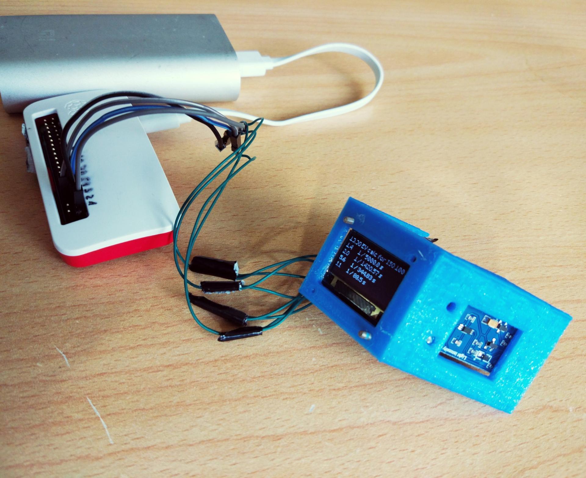
It looks like everything is working! The readout contains the light intensity in lux, EV value and also the ISO value for which it was calculated. Below you can see exposure times for given f stops. So what next? The problem with current script needs to be run from bash, and because Raspberry Pi Zero doesn’t have any input devices (mouse and keyboard), other computer or smartphone has to be involved to run the script and show measured values over ssh connection. Fortunately, there are small OLED displays compatible with Raspberry. Official ones from Adafruit are quite pricey (~19$) but there also available cheap Chinese copies which work with the same python libraries. I bought SSD1306 0.96″ OLED display 128×64 px for ~3$. To install the Adafruit library you should follow steps described on official Adafruit website: https://learn.adafruit.com/.
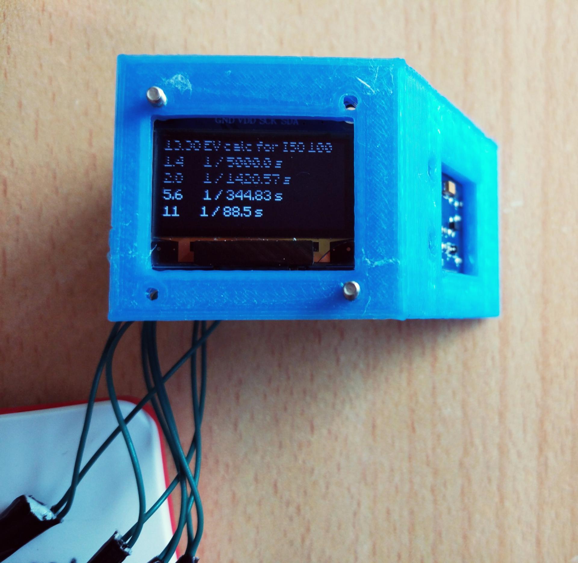
This display renders desired content but before the next one is loaded it has to be cleared with the black rectangle. This makes things slightly more complicated but with the proper understanding it is easy to solve. I joined my previous script for the light metering with Adafruit’s SSD1306 example script for Raspberry Pi usage statistics. Because the display area is very limited I had to reduce number of information displayed on the screen. I have chosen only 4 f stops: f/1.4, 2.0, 5.6, and 11 with refreshing rate 1 s. This is how the final code looks like:
#!/usr/bin/python
import math
from time import sleep

import Adafruit_SSD1306
from PIL import Image
from PIL import ImageDraw
from PIL import ImageFont
import smbus

# Raspberry Pi pin configuration:
RST = None  # on the PiOLED this pin isnt used
# 128x64 display with hardware I2C:
disp = Adafruit_SSD1306.SSD1306_128_64(rst=RST)

# Initialize library.
disp.begin()

# Clear display.
disp.clear()
disp.display()

# Create blank image for drawing.
# Make sure to create image with mode '1' for 1-bit color.
width = disp.width
height = disp.height
image = Image.new('1', (width, height))

# Get drawing object to draw on image.
draw = ImageDraw.Draw(image)

# Draw a black filled box to clear the image.
draw.rectangle((0, 0, width, height), outline=0, fill=0)

# Draw some shapes.
# First define some constants to allow easy resizing of shapes.
padding = -2
top = padding
bottom = height - padding
# Move left to right keeping track of the current x position for drawing shapes.
x = 0

font = ImageFont.truetype('Minecraftia.ttf', 8)

# Define some constants from the datasheet
DEVICE = 0x23  # Default device I2C address

POWER_DOWN = 0x00  # No active state
POWER_ON = 0x01  # Power on
RESET = 0x07  # Reset data register value

# Start measurement at 4lx resolution. Time typically 16ms.
CONTINUOUS_LOW_RES_MODE = 0x13
# Start measurement at 1lx resolution. Time typically 120ms
CONTINUOUS_HIGH_RES_MODE_1 = 0x10
# Start measurement at 0.5lx resolution. Time typically 120ms
CONTINUOUS_HIGH_RES_MODE_2 = 0x11
# Start measurement at 1lx resolution. Time typically 120ms
# Device is automatically set to Power Down after measurement.
ONE_TIME_HIGH_RES_MODE_1 = 0x20
# Start measurement at 0.5lx resolution. Time typically 120ms
# Device is automatically set to Power Down after measurement.
ONE_TIME_HIGH_RES_MODE_2 = 0x21
# Start measurement at 1lx resolution. Time typically 120ms
# Device is automatically set to Power Down after measurement.
ONE_TIME_LOW_RES_MODE = 0x23

bus = smbus.SMBus(1)  # Rev 2 Pi uses 1

def convertToNumber(data):
    # Simple function to convert 2 bytes of data
    # into a decimal number
    return ((data[1] + (256 * data[0])) / 1.2)

def readLight(addr=DEVICE):
    data = bus.read_i2c_block_data(addr, ONE_TIME_HIGH_RES_MODE_1)
    return convertToNumber(data)

def write_to_file(string):  # optional for export of the data
    import csv
    with open('light.csv', 'a') as fh:
        writer = csv.writer(fh)
        writer.writerow(string)

def iso_calc(iso):
    return 2 ** (math.log(iso / 100, 2))

def measure(iso):
    # f_stops = [1.4, 2, 2.8, 4, 5.6, 8, 11, 16, 22, 32, 45]   #full list of fstops
    f_stops = [1.4, 2, 2.8, 4, 5.6, 8, 11, 16, 22]

    while True:  # continues measurement
        light = round(readLight(), 2)  # get the light value from sensor

        if light > 0:
            draw.rectangle((0,0,width,height), outline=0, fill=0)
            draw.text((x, top), str(round(math.log((light) / 2.5, 2),2))+' EV calc for ISO '+str(iso), font=font, fill=255)
            draw.text((x, top+12), str(str(f_stops[0])+'       1 / '+str(round(1 / round(2.5 * f_stops[0] ** 2 / (float(light)) / iso_calc(iso),4),2))+' s'), font=font, fill=255)
            draw.text((x, top+24), str(str(f_stops[2])+'       1 / '+str(round(1 / round(2.5 * f_stops[2] ** 2 / (float(light)) / iso_calc(iso),4),2))+' s'), font=font, fill=255)
            draw.text((x, top+36), str(str(f_stops[4])+'       1 / '+str(round(1 / round(2.5 * f_stops[4] ** 2 / (float(light)) / iso_calc(iso),4),2))+' s'), font=font, fill=255)
            draw.text((x, top+48), str(str(f_stops[6])+'       1 / '+str(round(1 / round(2.5 * f_stops[6] ** 2 / (float(light)) / iso_calc(iso),4),2))+' s'), font=font, fill=255)

            # Display image.
            disp.image(image)
            disp.display()
            sleep(1)

measure(100)  # measure + iso value
I also changed the font to Minecraftia, because it uses much less space on the display. Unfortunately, when I was mounting the display to self-made holder it broke and first two rows are now showing all pixels. The prototype of the “case” for 3D printing can be downloaded from mine Thingverse profile: Light meter case prototype on Thingverse.
The only thing what still needs to be done is active change of ISO. Right now, ISO can be changed in the script by inserting the value to function measure (ISO). The perfect solution would be to have a knob which would change ISO value in the real time. The script should also auto-start with Raspberry and this can be easily done with crontab job:
sudo crontab -e

#add line as the last one

@reboot /home/pi/python light_meter_final.py
With those easy steps I showed you that it is possible to build a light meter at almost marginal costs (Raspberry Pi Zero ~12$ + GY-30 ~3$ + OLED ~3$ = 20$). Of course professional ones offer much better measuring range, more features and also different working modes but the idea of the project was to build something simple which would measure exposure in most standard conditions.